2019 H2 Math Paper 1 Question 9 Part (ib): the trigonometric approach

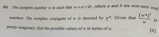
Show that $\displaystyle \frac{w-1}{w+1}$ can be expressed as $k \tan \frac{1}{2} \theta$, where $k$ is a complex number to be found.

In the video I introduced the “half-angle trick” using complex numbers in exponential/Euler form to solve the 2019 H2 Math Paper 1 Question 9 (ib). In this blog post I will illustrate a trigonometric approach.

The main key in a trigonometric approach involves the double angle formula: while the sine double angle is pretty straightforward $\sin 2A = 2 \sin A \cos A$, there are 3 different version of the cosine double angle formula $\cos 2A = \cos^2 A – \sin^2 A = 2 \cos^2 A – 1 = 1 – 2 \sin^2 A$. For this question (and in some other applications), the trick is to use the appropriate formula to eliminate any “1”s in the question. For example, in our working we will encounter $\cos \theta – 1$. If we let $\cos \theta = 1 – 2 \sin^2 \frac{\theta}{2}$, then $\cos \theta – 1 = 1 – 2 \sin^2 \frac{\theta}{2} – 1 = -2 \sin^2 \frac{\theta}{2}$, so the “$-1$” was eliminated. Similarly, when dealing with $\cos \theta + 1$, we want to use the other variant of the double angle formula to get $\cos \theta + 1 = 2 \cos^2 \frac{\theta}{2} – 1 + 1 = 2 \cos^2 \frac{\theta}{2}$.

The solution:

\begin{align}
\frac{w-1}{w+1}
&= \frac{\cos \theta + i \sin \theta – 1}{\cos \theta + i \sin \theta + 1} \\
&= \frac{1 – 2 \sin^2 \frac{\theta}{2} + i 2 \sin \frac{\theta}{2} \cos \frac{\theta}{2} – 1}{2\cos^2 \frac{\theta}{2} – 1 + i 2 \sin \frac{\theta}{2} \cos \frac{\theta}{2} + 1} \\
&= \frac{- 2 \sin^2 \frac{\theta}{2} + 2i \sin \frac{\theta}{2} \cos \frac{\theta}{2}}{2\cos^2 \frac{\theta}{2} + 2i \sin \frac{\theta}{2} \cos \frac{\theta}{2}} \\
&= \frac{2 \sin \frac{\theta}{2} (- \sin \frac{\theta}{2} + i \cos \frac{\theta}{2})}{2 \cos \frac{\theta}{2} (cos \frac{\theta}{2} + i \sin \frac{\theta}{2})} \\
&= \tan \frac{\theta}{2} \frac{- \sin \frac{\theta}{2} + i \cos \frac{\theta}{2}}{cos \frac{\theta}{2} + i \sin \frac{\theta}{2}} \times \frac{\cos \frac{\theta}{2}-i\sin \frac{\theta}{2}}{\cos \frac{\theta}{2}-i\sin \frac{\theta}{2}} \\
&= \tan \frac{\theta}{2} \frac{-\sin \frac{\theta}{2} \cos \frac{\theta}{2} +i\sin^2 \frac{\theta}{2} + i \cos^2 \frac{\theta}{2} -i^2 \sin \frac{\theta}{2} \cos \frac{\theta}{2}}{\cos^2 \frac{\theta}{2}+\sin^2 \frac{\theta}{2}} \\
&= \tan \frac{\theta}{2} \frac{-\sin \frac{\theta}{2} \cos \frac{\theta}{2} + \sin \frac{\theta}{2} \cos \frac{\theta}{2} +i(\sin^2 \frac{\theta}{2} +\cos^2 \frac{\theta}{2}) }{1} \\
&= \left ( \tan \frac{\theta}{2} \right) i
\end{align}

Hence $k= i$.

spacer

Behind the curtain

A brief glimpse “behind the curtain”: the setup I use during zoom video classes!

The lockdown/circuit breaker sure has brought its shares of challenges in teaching and learning. Lessons are certainly slightly less effective without the physical interactive component: I can’t just look over students’ shoulder and check on their progress, and it’s definitely been harder to gauge how my explanations are faring without the feedback from non-verbal cues. Not to mention the occasional lag and technical difficulties.

spacer

Still climbing onto the shoulders of giants

It was year 2005/2006: I was taking further maths in JC under Mr Wee when he showed some video clips about linear algebra (what we were learning about at that time) to us during lecture. In addition to the math content I also remembered how he told us about this initiative by MIT, the OpenCourseWare, where some course content (including video lectures) from the university were being uploaded and made available for free to the public. Thinking back, this was pretty remarkable (youtube was still in its infancy). I recall at that time, finding the experience pretty interesting (MIT is nerd heaven after all, so there’s the brand name recognition. Plus the video lecture was challenging but engaging: something I’d sure hope to experience when I get to university), but that’s about it. After all, who has time during JC do much more on top of academic and social life!

spacer

Alternative method to find food of perpendicular (without using vector projections)

In my video (link to be updated) I have worked out examples of how to use projection vectors to find the foot of perpendicular (for both lines and planes). The benefits of this method

  1. it is faster,
  2. it uses a similar concept for both lines and planes with slight modifications.

The downsides, however, is that it involves a rather unwieldy projection vector formula $(\mathbf{a}\cdot\mathbf{\hat{b}}) \mathbf{\hat{b}}$ and that minor details make a huge difference to whether we get the correct answer (e.g. where are our vectors pointing, $\overrightarrow{AB}$ or $\overrightarrow{BA}$? Is our final projection vector $\overrightarrow{AF}$ or $\overrightarrow{FB}$?).
In this post I will offer an alternative method to find foot of perpendicular using earlier concepts that some students find easier to understand.


Finding foot of perpendicular to a line

spacer

Q9b discussion

The integration part

We have $\displaystyle \int \frac{1}{(1-x^2)(1+x^2)} \; \mathrm{d}x = t + C$. Since the denominator is so complicated, partial fractions is the way to go.
$$ \frac{1}{(1-x)(1+x)(1+x^2)} = \frac{A}{1-x} + \frac{B}{1+x} + \frac{Cx+D}{1+x^2}.$$
Give it a go!

spacer

Q6b discussion

Using your method

Continuing from your method (making sure to use a new letter), we have $$ \frac{a^2-b^2-2abi}{a+bi} = 0 + ic$$ Simplifying gives us $a^2-b^2 - 2abi = -bc + aci$. It looks very unwieldy, but let's use our usual techniques (comparing real and imaginary parts). Our final aim is to find $w$ in terms of $a$ so let's find $b$ and $c$ in terms of $a$. Give it a try first, and you can check against my working below:

spacer

Q3i discussion

Turns out for this question we don't need to use formulas like volume of hemisphere, etc.

Instead, we are given an equation of a curve $x^2 + (y-5)^2 = 25$. We want the volume of the water in the bowl. Able to spot which topic can help us tackle that?

spacer

Alternative method to find the line of intersection between two planes

In the video (link to be updated), we went through how to find the line of intersection between two planes using a GC. In this post, we will discuss an alternative method to accomplish this without the use of technology. Just like in our video, we will use the following example:
Find the equation of the line of intersection between $$ p_1: \mathrm{r} \cdot \begin{pmatrix} 1 \\ 0 \\ 5 \end{pmatrix} = 7, \quad p_2: \mathrm{r} \cdot \begin{pmatrix} 1 \\ 1 \\ -1 \end{pmatrix} = -3.$$
The two important things we need to find an equation for a line are (1) a point on the line and (2) the direction vector parallel to the line. We will thus tackle the two separately:

Finding the direction vector

The key observation here is that the direction vector of the line of intersection is perpendicular to the normal vectors of both planes (try to visualize it!). Thus, to find the direction vector of the line of intersection, we can use the cross product. Hence
spacer

Why $\mathbf{r}\cdot\mathbf{n} = \mathbf{a}\cdot\mathbf{n}$ for planes?

When I was first learning about equations of planes, the vector form of a plane $\mathbf{r} = \mathbf{a} + \lambda \mathbf{d_1} + \mu \mathbf{d_2}$ made a lot more sense to me: pick different values of $\lambda$ and $\mu$, and we will end up at different points on the plane.

And while I can see why the vector form isn’t as useful for further applications because there are so many different direction vectors (infinite, in fact), and that the normal vector is a much better way to describe planes because it is unique (up to a scalar multiple), the equation $\mathbf{r}\cdot\mathbf{n} = \mathbf{a}\cdot\mathbf{n}$ just isn’t very intuitive and didn’t make a lot of sense. In today’s post I’d try my best to explain the origins of such an equation.

Understanding how the equation comes about boils down to knowing what $\mathbf{a}$ and $\mathbf{r}$ represent. $\mathbf{a}$ is the position vector of a fixed point $A$ that we already know lies on the plane. In forming an equation of an object, we will like to know what equation any other random points on the object satisfies. (For example, we say $y=2x+3$ is an equation of a line because we can check that $(0,3)$ satisfies the equation (and hence lies on the line) while $(1,4)$ does not). $\mathbf{r}$ is used to represent the position vector of a random point on our plane. We will call the point $R$.

So, in the picture above, we have fixed $A$, and randomly pick a few points which we named $R_1, R_2$ and $R_3$. It turns out that, regardless of which $R$ we take, we can form a direction vector $\overrightarrow{AR}$. And the normal vector of our plane, $\mathbf{n}$ is so special in the sense that $\overrightarrow{AR}$ is perpendicular to $\mathbf{n}$. Thus we have $\overrightarrow{AR} \cdot \mathbf{n} = 0$.

The rest boils down to some algebra manipulation. $\overrightarrow{AR} = \overrightarrow{OR}-\overrightarrow{OA}$ so $(\mathbf{r}-\mathbf{a})\cdot \mathbf{n} = 0$. Expansion gives $\mathbf{r} \cdot \mathbf{n} – \mathbf{a} \cdot \mathbf{n} = 0$ which leads us to our familiar $\mathbf{r}\cdot\mathbf{n} = \mathbf{a}\cdot\mathbf{n}$.

Hopefully this proof and explanation helps, but I bet that even then the equation still looks a bit weird (it did to me years ago too!). The trick is to simply keep practicing with it and it’d become second nature in no time!

spacer

Proofs of common number properties

I will name some properties I will use for future references with MP (my proposition) below:

(MP1.1) 0 times anything is 0

Let $a$ be any number. Let’s start with $a \cdot 0$. By the property of $0$, we have $a \cdot 0 = a \cdot (0 + 0)$. Using the distributive property gives us $a \cdot 0 + a \cdot 0$. Combining it all together we have $a\cdot 0 = a\cdot 0 + a\cdot 0$. But the definition of $0$ is such that it doesn’t change a number after addition. So $a \cdot 0 = 0$.

(MP1.2) $(-a)b = – (ab)$

Note the meaning of $-a$ is the additive inverse of $a$, meaning that $a + (-a) = 0$ while the meaning of $-(ab)$ is the additive inverse of $ab$. Let’s add $ab$ with $(-a)b$.
$ab + (-a)b = (a + (-a)) \cdot b$ by the commutative and distributive laws. Since $-a$ is the additive inverse of $a$, this gives us $0 \cdot b$ which is $0$ from MP1.1. Thus $(-a)b$ is the additive inverse of $ab$ which is what we want to prove.

(MP1.3) $(-a)(-b) = ab$

$ (-a)(-b) + -(ab) = (-a)(-b) + (-a)(b)$ by the MP1.2. By the distributive property, $(-a)(-b) + (-a)b = (-a)(-b + b) = (-a)0 = 0$ by MP1.1. Since $-(ab)$ is the additive inverse of $ab$, $(-a)(-b)$ must have been $ab$.

We cannot have the multiplicative inverse of 0

Suppose there exist the multiplicative inverse of $0$, which we will denote by $0^{-1}$. Then $0 \cdot 0^{-1} = 1$. But by MP1.1, $0$ times anything is 0 so $0=1$. This brings us a whole host of problems: $1 + 1 = 0 + 0 = 0$. So no matter what we do, every number we try to create will all become 0. Hence allowing the multiplicative inverse of 0 means that we can only work with one number: not a very interesting proposition. Conversely, to have more than one number to work with, we cannot allow the multiplicative inverse of 0.

(MP1.4) Corollory of $(-a)b = -(ab): (-1)b = -b$

(MP1.5) If $ab=0$, then $a=0$ or $b=0$.

Case 1: $a=0$. That is part of the solution.
Case 2: $a \neq 0$. Then the multiplicative inverse $a^{-1}$ exists. So $ab= 0$ means $a^{-1} ab = a^{-1} 0 $ so $b=0$.

(MP1.6) $(ab)^{-1} = a^{-1}b^{-1}$

$ab (a^{-1}b^{-1}) = a a^{-1} b b^{-1}$ by the commutative and associative properties which gets us $1 \cdot 1 = 1$ by the property of the multiplicative identity $1$. Hence $a^{-1}b^{-1}$ is the multiplicative inverse of $ab$.

spacer